2 Methods
We defined the terms “order event and”reconstruction" strictly, developed a software that reconstructs order events in accordance with these definitions from data provided by several cryptocurrency exchanges and analysed whether the exchanges provide enough information for the comprehensive reconstruction of their order book evolution.
Surprisingly, an order, an order event, a limit order book, the operations of a continuous double auction are rather complicated things if one attempts to define them rigorously. Consider, for example, a definition given in the book (Bouchaud and Bonart 2018):
An order is a commitment, declared at a given submission time, to buy or sell a given volume of an asset at no worse than a given price. An order \(x\) is thus described by four attributes:
- its sign (or direction) \(\epsilon = \pm 1\), (\(\epsilon_x = +1\) for buy orders; \(\epsilon_x = −1\) for sell orders),
- its price \(p_x\) ,
- its volume \(v_x > 0\), and
- its submission time \(t_x\).
We introduce the succinct notation \(x := (\epsilon_x , p_x ,v_x, t_x )\).
(Bouchaud and Bonart 2018) then continues with a description of what they call The Trade-Matching Algorithm:
Whenever a trader submits a buy (respectively, sell) order \(x\), an LOB’s trade-matching algorithm checks whether it is possible for \(x\) to match to existing sell (respectively,buy)orders \(y\) such that \(p_y \leq p_x\) (respectively, \(p_y \geq p_x\)). If so, the matching occurs immediately and the relevant traders perform a trade for the agreed amount at the agreed price. Any portion of \(x\) that does not match instead becomes active at the price \(p_x\), and it remains active until either it matches to an incoming sell (respectively, buy) order or it is cancelled. Cancellation usually occurs when the owner of an order no longer wishes to offer a trade at the stated price.
The above definition and description are incomplete:
According to the definition, an order \(x\) seems to be an immutable entity. But according to the Trade-Matching algorithm, a portion of \(x\) may become ‘active’ and it is not clear how the quality of being ‘active’ is different from the mere existence of submitted orders,
At what price the trade is performed - \(p_x\) or \(p_y\) - is not explicitly stated,
It is not stated what will happen if \(v_x \leq v_y\), etc.
Below we propose stricter definitions that address these and the other similar issues trying to stay close to (Bouchaud and Bonart 2018). Afterwards we describe the reconstruction process.
2.1 Definitions
2.1.1 Order function
Definition 2.1 (Order Function) A function \(o : \mathbb{R}_{>0} \times \mathbb{R} \mapsto \mathbb{R}\) is called a limit order function if it can be written as \[ o(p,t) = \sum_{k=1}^K v_k \mathbf{1}_{P_k \times T_k}(p,t) \] where
- \(\mathcal{T} = \{T_k\}_{k=1}^{K}\) is a partition of left-open finite or right-unbounded interval of \(\mathbb{R}\) into intervals with endpoints \(t_{k,1} \in \mathbb{R}\), \(t_{k,2} \in \mathbb{R} \cup \{+\infty\}\) such that:
- \(\forall k \leq K : t_{k,1},t_{k,2} \in \{n \tau : n \in \mathbb{Z}\}\), where \(\tau \in \mathbb{R}_{>0}\) is a constant called sampling interval
- \(\forall k < K : t_{k,1} \leq t_{k+1,1} \land t_{k,2} < t_{k+1,2}\)
- \(\mathcal{P} = \{P_k\}_{k=1}^{K}\) is a set of degenerate intervals \(P_k = \{p_k\}\) with endpoints \(p_k \in \mathbb{R}_{> 0}\), such that:
- \(\forall k: p_k \in \{ n \pi : n \in \mathbb{N} \}\) where \(\pi \in \mathbb{R}_{>0}\) is a constant called quote increment or tick size,
- \(\forall k < K\) if \(t_{k,2} \not \in T_k\) then \(p_{k+1} = p_k\)
- \(\mathcal{V} = \{v_k \}_{k=1}^K\) is a set of constants \(v_k \in \mathbb{R}_{\neq 0}\) called order volumes such that:
- \(\forall k\) either \(v_k \in \mathbb{R}_{> 0}\) (buy order) or \(v_k \in \mathbb{R}_{< 0}\) (sell order),
- \(|v_k| \in \{ n \phi : n \in \mathbb{N}\}\) where \(\phi \in \mathbb{R}_{>0}\) is a constant called base increment or lot size,
- \(\mathbf{1}_{P_k \times T_k}(p, t)\) is an indicator function of the set \({P_k \times T_k}\): \[ \mathbf{1}_{P_k \times T_k}(p,t) = \begin{cases} 1, & (p,t) \in P_k \times T_k \\ 0, & (p,t) \not \in P_k \times T_k \end{cases} \]
The sample interval \(\tau\), quote increment \(\pi\) and base increment \(\phi\) are collectively called resolution parameters.
Definition 2.4 (Filled Volume) Suppose a volume function \(v(t)\) as defined by 2.3 is given. The function \[ f_{v}(t) = v(t) - \lim_{t^{'} \uparrow t} v(t^{'}) \] is called a filled volume at time \(t\).
\(f_{v}(t) \neq 0\) implies that there is a right-open interval \(T_k\) such that its right endpoint equals to \(t\).
Definition 2.5 (Amended Volume) Suppose a volume function \(v(t)\) as defined by 2.3 is given. The function \[ a_{v}(t) = \lim_{t^{'} \downarrow t} v(t^{'}) - v(t) \] is called an amended volume at time \(t\).
It follows from definition 2.1 that \(T_1\) is left-open, so \(a_v(t_{1,1}) = v_1 \neq 0\). This is the only place where we follow (Bouchaud and Bonart 2018) by modelling order placement as càglàd (continue à gauche, limite à droite) process:
… we will consider the evolution of an LOB \(\mathcal{L}(t)\) as a so-called càglàd process (continu à gauche, limite à droite). Informally, this means that when a new order \(x\) is submitted at time \(t_x\) , we regard it to be present in the LOB immediately after its arrival, but not immediately upon its arrival.
Then \(a_v(t) \neq 0\) at some point \(t_{1,1} < t < t_{K,2}\) implies that there is a left-open interval \(T_k\) such that its left endpoint equals to \(t\).
Finally \(a_{v}(t_{K,2}) \neq 0\) implies that \(T_K\) is a right-closed, possibly degenerate, interval.
An order can be conveniently represented in the form of a order table defined by 2.7.
Definition 2.6 (Order Event) An order event is a tuple \((t,s,p,v,m)\) where
- \(t \in \mathbb{R}\) is an event timestamp
- \(s \in \{0, 1\}\) is the state of the order after the event; \(s = 1\) means the order is active; \(s = 0\) means that order is done (finished) i.e. removed from an order book,
- \(p \in \mathbb{R}_{>0}\) is the order price,
- \(v \in \mathbb{R}\) is the order volume,
- \(m \in \{0,1\}\) is a match indicator; \(m =1\) means that the order has been matched with another one and a trade has occurred between them so the event has been originated by the trade; \(m = 0\) means that the event is an amendment and has not been originated by a trade.
Definition 2.7 (Order Table) Suppose an order function \(o(p,t)\) as defined by 2.1 is given. A set \[\mathcal{E} = \{(t_k',s_k',p_k',v_k', m_k')\}_k\] of \(K\) or \(K+1\) order events
\(\forall k \in \{1, \ldots, K\}\) \(k\)’s order event is defined as follows:
- \(t_k' = t_{k,1}, s_k' = 1, p_k' = p_k, v_k' = v_k\),
- if \(t_{k,1} \in T_k\) then \(m_k' = 1\), otherwise \(m_k' = 0\),
if \(T_K\) is a finite interval, then \(K+1\)’s order event is defined as follows:
- \(t_{K+1}' = t_{K,2}, s_{K+1}' = 0, p_{K+1}'=p_K\),
- if \(t_{K,2} \not \in T_K\) then \(m_{K+1} = 1\),\(v_{K+1}' = 0\); otherwise \(m_{K+1}' = 0\), \(v_{K+1}' = v_k\)
is called an order table. The index \(k\) is called an event ordinal number.
Proof. Suppose the order table \(\mathcal{E} = \{(t_k',s_k',p_k',v_k', m_k')\}_{k=1}^{R}\) is given. To restore the corresponding order function \(o(p,t)\) as defined by 2.1 we need to restore \(\mathcal{T}\), \(\mathcal{P}\) and \(\mathcal{V}\) sets. It can be done as follows:
For all \(1 \leq k < R\)
The interval \(T_k\) with left endpoint \(t_k'\) and right endpoint \(t_{k+1}'\) which is:
- a left-open if \(m_k'=0\) and left-closed if \(m_k'=1\)
- a right-open if \(m_{k+1}'=1\) and right-closed if \(m_{k+1}'=0\)
is added to \(\mathcal{T}\)
The interval \(P_k = \{p_k'\}\) is added to \(\mathcal{P}\)
The constant \(v_k'\) is added to \(\mathcal{V}\)
If \(s_R' = 1\):
- The interval \(T_R\) which is either \((t_R', +\infty)\) if \(m_R'=0\) or \([t_{R}', +\infty)\) if \(m_R'=1\) is added to \(\mathcal{T}\),
- The interval \(P_R = \{p_R\}\) is added to \(\mathcal{P}\),
- The constant \(v_R'\) is added to \(\mathcal{V}\); note that \(v_R' \neq 0\).
Note that \(|\mathcal{E}| = |\mathcal{T}| + 1\) if the last interval \(T_k\) is finite and \(|\mathcal{E}| = |\mathcal{T}|\) otherwise, as in definition 2.7.
See Appendix for examples of order tables and order functions restored from them.
2.1.2 Order book
Typically the term order book refers to an electronic list of buy and sell orders for a specific security or financial instrument organized by price level. An order book lists the number of shares being bid on or offered at each price point, or market depth. Order books are used by almost every exchange to list the orders for different securities.
From definition of an order 2.1 follows that \(\mathcal{O} = \mathcal{A} \cup \mathcal{B}\) and \(\mathcal{A} \cap \mathcal{B} = \emptyset\).
To make the above definitions intuitively clear, consider an example in Appendix.
Note that \[\text{supp}(o^{\mathcal{A}}(p,t)) \cap \text{supp}(o^{\mathcal{B}}(p,t)) = \emptyset\] but \(\overline{\text{supp}(o^{\mathcal{A}}(p,t))} \cap \overline{\text{supp}(o^{\mathcal{B}}(p,t))}\) may be non-empty and in this case it will be a finite set of points.
2.1.3 Market orders
A market order is a request by an investor to buy or sell a security at the best available price at the time of order placement. The request is usually made through a broker or brokerage service and is ultimately executed by an exchange that maintains an order book. Clearly, a market order cause an exchange’s order book to be updated so market orders are modeled as changes of an order book.
Definition 2.17 (Market Buy Order) Suppose a Limit Order Book \(\mathcal{L}\) is given as defined by 2.15. Suppose that at time \(t_j\) \[\sum_{o^a(\cdot, \cdot) \in \mathcal{A(t_j)} } f_{v^a}(t_j) < 0 \] Then it is said that a market buy order is placed and executed at time \(t_j\) for \(\sum_{o^a(\cdot, \cdot) \in \mathcal{A}(t_j) } |f_{v^a}(t_j)p^a(t_j)|\) units of currency.
Definition 2.18 (Market Sell Order) Suppose a Limit Order Book \(\mathcal{L}\) is given as defined by 2.15. Suppose that at time \(t_j\) \[\sum_{o^b(\cdot, \cdot) \in \mathcal{B}(t_j) } f_{v^b}(t_j) > 0 \] Then it is said that a market sell order is placed and executed at time \(t_j\) for \(\sum_{o^b(\cdot, \cdot) \in \mathcal{B}(t_j) } f_{v^b}(t_j)\) units of asset.
2.1.4 Level2 order function
The Order Set Table is a precise representation of Order Functions but it is not a good tool for analysis. Consider for example the really short table 2.1. Even in this simple case, it is rather hard to see how LOB was evolving. The visual representation of the same Order Set Tableshown on figure 2.1 is much more expressive.
| \(i\) | \(k\) | \(t^i_k\) | \(s^i_k\) | \(p^i_k\) | \(v^i_k\) | \(m^i_k\) |
|---|---|---|---|---|---|---|
| 1 | 1 | 2021-03-26 13:59:06.0 | 1 | 535 | 0.9 | 0 |
| 2 | 1 | 2021-03-26 13:59:06.2 | 1 | 530 | 1 | 0 |
| 3 | 1 | 2021-03-26 13:59:06.4 | 1 | 540 | -0.5 | 0 |
| 1 | 2 | 2021-03-26 13:59:06.8 | 1 | 535 | 0.3 | 1 |
| 3 | 2 | 2021-03-26 13:59:07.0 | 0 | 540 | 0 | 1 |
| 1 | 3 | 2021-03-26 13:59:07.2 | 0 | 535 | 0.3 | 0 |
| 2 | 2 | 2021-03-26 13:59:07.2 | 0 | 530 | 1 | 0 |
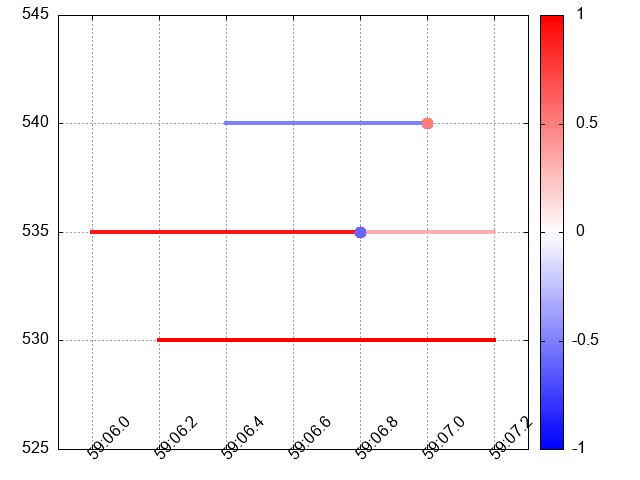
Figure 2.1: It is easier to grasp the evolution of an order book from the visual representation of Order Set Table 2.1 shown above
Unfortunately, not every Order Set Table can be visualised ‘as-is.’ Suppose that one more order function is added to LOB as shown in table 2.2. Its visualisation shown on figure 2.2 is distorted since the lines corresponding to orders 3 and 4 overlaps. These orders have the same price and their time intervals intersects.
| \(i\) | \(k\) | \(t^i_k\) | \(s^i_k\) | \(p^i_k\) | \(v^i_k\) | \(m^i_k\) |
|---|---|---|---|---|---|---|
| 1 | 1 | 2021-03-26 13:59:06.0 | 1 | 535 | 0.9 | 0 |
| 2 | 1 | 2021-03-26 13:59:06.2 | 1 | 530 | 1 | 0 |
| 3 | 1 | 2021-03-26 13:59:06.4 | 1 | 540 | -0.5 | 0 |
| 4 | 1 | 2021-03-26 13:59:06.6 | 1 | 540 | -1 | 0 |
| 1 | 2 | 2021-03-26 13:59:06.8 | 1 | 535 | 0.3 | 1 |
| 3 | 2 | 2021-03-26 13:59:07.0 | 0 | 540 | 0 | 1 |
| 1 | 3 | 2021-03-26 13:59:07.2 | 0 | 535 | 0.3 | 0 |
| 2 | 2 | 2021-03-26 13:59:07.2 | 0 | 530 | 1 | 0 |
| 4 | 2 | 2021-03-26 13:59:07.2 | 0 | 540 | -1 | 0 |
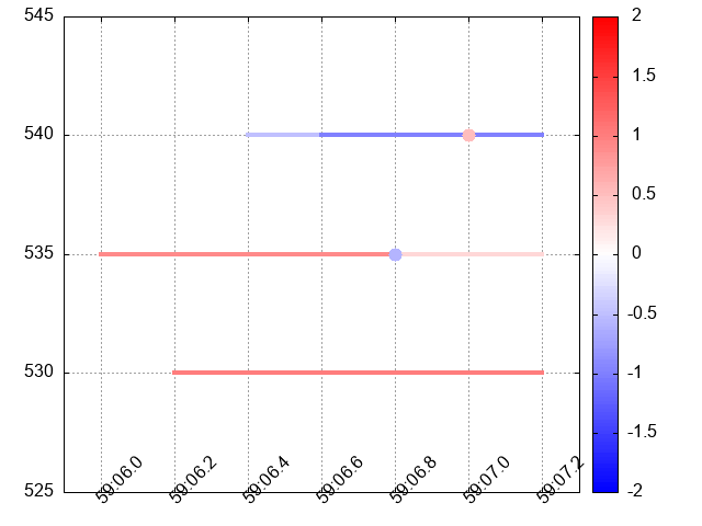
Figure 2.2: A visual representation of Order Book Set 2.2 is distorted since the lines representing orders 3 and 4 overlap
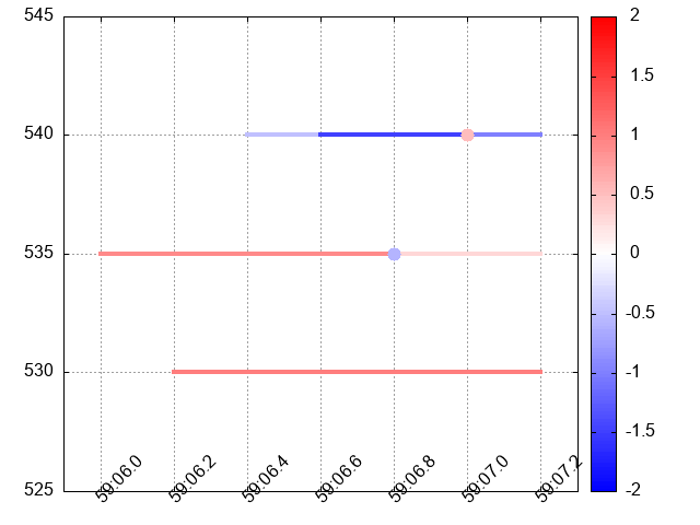
This example is a motivation for theorem 2.2. The theorem guarantees that we may transmute Order Set Table into another one, which at every moment and for every price contains only one non-zero order function.
Theorem 2.2 (Level2 Order Function) Suppose Limit Order Book \(\mathcal{L}\) as defined by 2.15 is given, \(o^{\mathcal{L}}(p,t)\) is LOB function as defined by 2.16 (either LOB bid function or LOB ask function) and for some constant \(p_0 \in \mathbb{R}_{>0}\): \[\emptyset \neq \text{supp}(o^{\mathcal{L}}(p_0,t)) = \bigcup_{m=1}^M I_m\] where all \(I_m\) are intervals such that \(\forall i,j: \overline{I_i} \cap \overline{I_j} = \emptyset\).
Then \(\forall m: m \in [1, \ldots, M]\) Level2 Order Function \(o^{p_0, m}(p,t)\) defined as:
\[ o^{p_0, m}(p,t) = \begin{cases}o^{\mathcal{L}}(p_0,t), & (p,t) \in \{p_0\} \times I_m \\ 0, & \text{otherwise} \end{cases} \] is Order Function as defined by 2.1.Proof. To prove the theorem we need to construct \(\mathcal{T}\), \(\mathcal{P}\) and \(\mathcal{V}\) sets which are used in definition 2.1.
Suppose that \(\{t_r^m\}_{r=1}^R \in I_m\) are points of dicontinuity of \(o^{p_0,m}(p_0,t)\).
If \(R=1\) then \(\mathcal{T} = \{(t^m_1, +\infty)\}\), \(\mathcal{P} = \{\{p_0\}\}\), \(\mathcal{V} = \{o^{p_0,m}(p_0,t^m_1)\}\).
Now suppose that \(R >1\). We may assume without loss of generality that \(t^m_i < t^m_j\) if \(i < j\). Then \(\forall r \in \{1, \ldots, R\}\) we’ll construct \(T_r \in \mathcal{T}\), \(P_r \in \mathcal{P}\), \(v_r \in \mathcal{V}\) as follows:
- \(P_r = \{p_0\}\),
- \(v_r = o^{p_0, m}(p_0, \frac{t_r+t_{r+1}}{2})\),
- \(T_r\) is an interval with left endpoint \(t_r\) and right-endpoint \(t_{r+1}\); it is left-closed if \(o^{p_0,m}(p_0, t_r) = v_r\) and left-open otherwise; it is right-closed if \(o^{p_0,m}(p_0, t_{r+1}) = v_r\) and right-open otherwise,
If \(I_m\) is right-unbounded then \(T_{R+1}\) with \(t_R\) as its left-endpoint and \(+\infty\) as its right-endpoint is added to \(\mathcal{T}\), \(P_{R+1} = \{p_0\}\), \(v_{R+1} = o^{p_0, m}(p_0, t_R+1)\); \(T_{R+1}\) is left-closed if \(o^{p_0,m}(p_0, t_R) = v_{R+1}\) and left-open otherwise.
Finally, \(\forall t^m_r : r > 1 \land t^m_r \not \in T_{r-1} \land t^m_r \not \in T_r\) a degenerate interval \(\{t^m_r\}\) is added to \(\mathcal{T}\), corresponding interval \(\{p_0\}\) is added to \(\mathcal{P}\) and corresponding value \(o^{p_0, m}(p_0, t^m_r)\) is added to \(\mathcal{V}\).
Table 2.3 is a transmuted table 2.2. Its visual representation shown on figure 2.3 is not distorted since order 5, which is Level2 Order Function, properly aggregates volumes of orders 3 and 4.
| \(i\) | \(k\) | \(t^i_k\) | \(s^i_k\) | \(p^i_k\) | \(v^i_k\) | \(m^i_k\) |
|---|---|---|---|---|---|---|
| 1 | 1 | 2021-03-26 13:59:06.0 | 1 | 535 | 0.9 | 0 |
| 2 | 1 | 2021-03-26 13:59:06.2 | 1 | 530 | 1 | 0 |
| 5 | 1 | 2021-03-26 13:59:06.4 | 1 | 540 | -0.5 | 0 |
| 5 | 2 | 2021-03-26 13:59:06.6 | 1 | 540 | -1.5 | 0 |
| 1 | 2 | 2021-03-26 13:59:06.8 | 1 | 535 | 0.3 | 1 |
| 5 | 3 | 2021-03-26 13:59:07.0 | 1 | 540 | -1 | 1 |
| 1 | 3 | 2021-03-26 13:59:07.2 | 0 | 535 | 0.3 | 0 |
| 2 | 2 | 2021-03-26 13:59:07.2 | 0 | 530 | 1 | 0 |
| 5 | 4 | 2021-03-26 13:59:07.2 | 0 | 540 | -1 | 0 |
2.2 Software
2.2.1 Main
main function of the application is rather short:
int main(int argc, char **argv) {

  oberon::Main app;
  return app.main(argc, argv);
}
Figure 2.4 shows the specification of oberon::App::main operation in the form of UML2 Activity Diagrams (Cook et al. 2017) of activity Main.
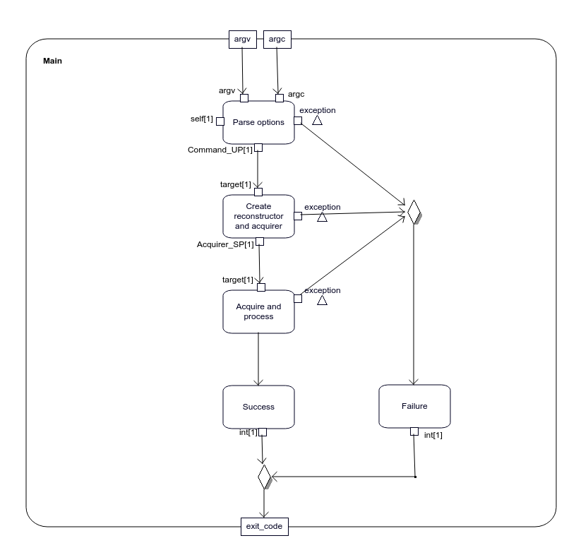
Figure 2.4: Activity Main - the specification of oberon::App::main operation.
CallOperationAction Parse options calls Main::parseOption operation that parse command-line options and returns an instance of a class derived from Command shown on figure 2.5 in light-green as determined by the value of “command” parameter passed.
CallOperationAction Create reconstructor and acquirer then calls operation Command::createAcquirer using the received Command-derived instance as a target. The overriden createAcquirer operation returns an appropriate instance of class derived from Acquirer shown on figure 2.6 in light-green.
The Acquirer-derived instance is then used as a target by CallOperationAction AcquireAndProcess that calls Acquirer::acquireAndProcess operation.
There are two kinds of acquireAndProcess operation. Their specifications are shown on figures 2.10 and 2.11. The former is used when Create reconstructor and acquirer returns an instance derived from Receiver class and the latter is used when the instance is derived from Reader class as shown on figure 2.6.
Upon successful completion of acquireAndProcess operation, ValueSpecificationAction Success returns EXIT_SUCCESS constant.
Otherwise, if some exception was raised, ValueSpecificationAction Failure returns EXIT_FAILURE constant.
Main activity is then completes.
2.2.2 Parse options
Action node “Parse options” on figure 2.4 returns a unique_ptr to an instance of concrete class (shown on figure 2.5 in light green) derived from the abstract class Command. As it can bee seen the concrete class is derived either from Capture or from Transform.
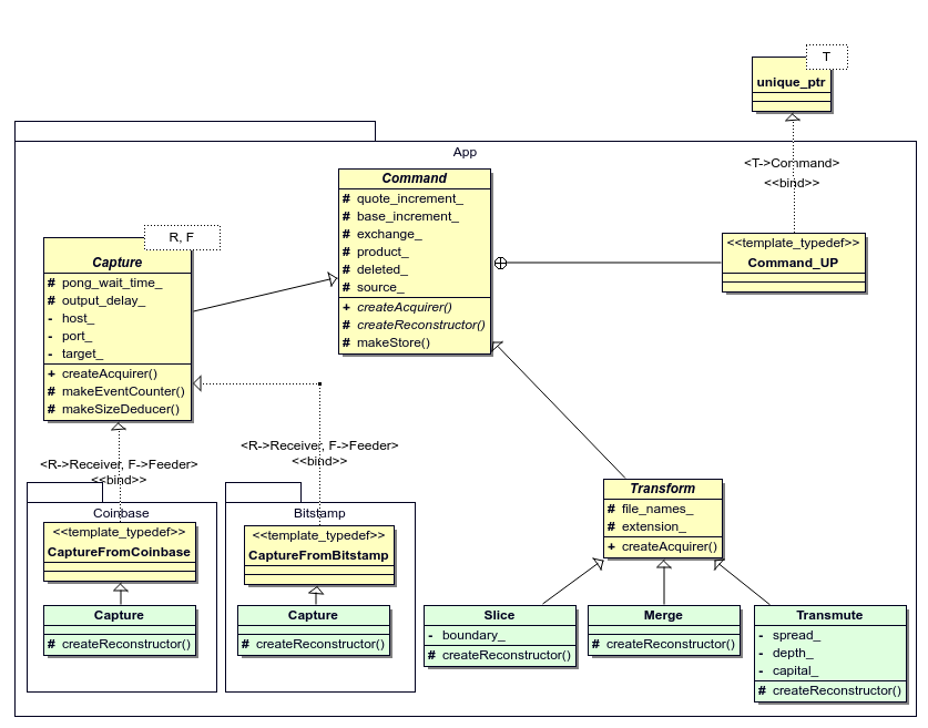
Figure 2.5: Command class hierarchy
2.2.3 Create reconstructor and acquirer
2.2.3.1 Create acquirer
Action node “Create reconstructor and acquirer” on figure 2.4 calls createAcquirer() method on the instance of Command class received on target input pin. The method calls the protected createReconstructor() method internally and returns a shared_ptr to an instance of concrete class derived from the abstract class Acquirer shown on figure 2.6 in light green.
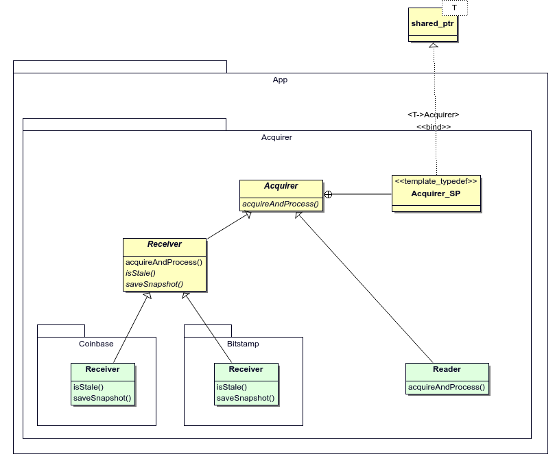
Figure 2.6: Acquirer class hierarchy
The specification of Receiver::acquireAndProcess operation is provided in section 2.2.4.1. The specification of Reader::acquireAndProcess operation is provided in section 2.2.4.2.
2.2.3.2 Create reconstructor
This section provides specifications of createReconstructor operation of concrete classes shown on figure 2.5 in light-green.
2.2.3.2.1 coinbase::Capture
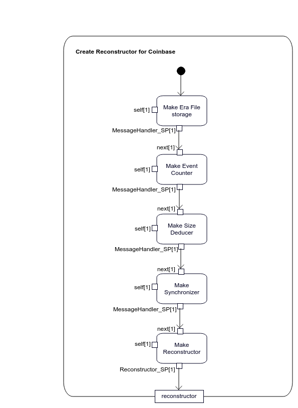
Figure 2.7: Specification of coinbase::Capture::createReconstructor operation
2.2.3.2.2 bitstamp::Capture
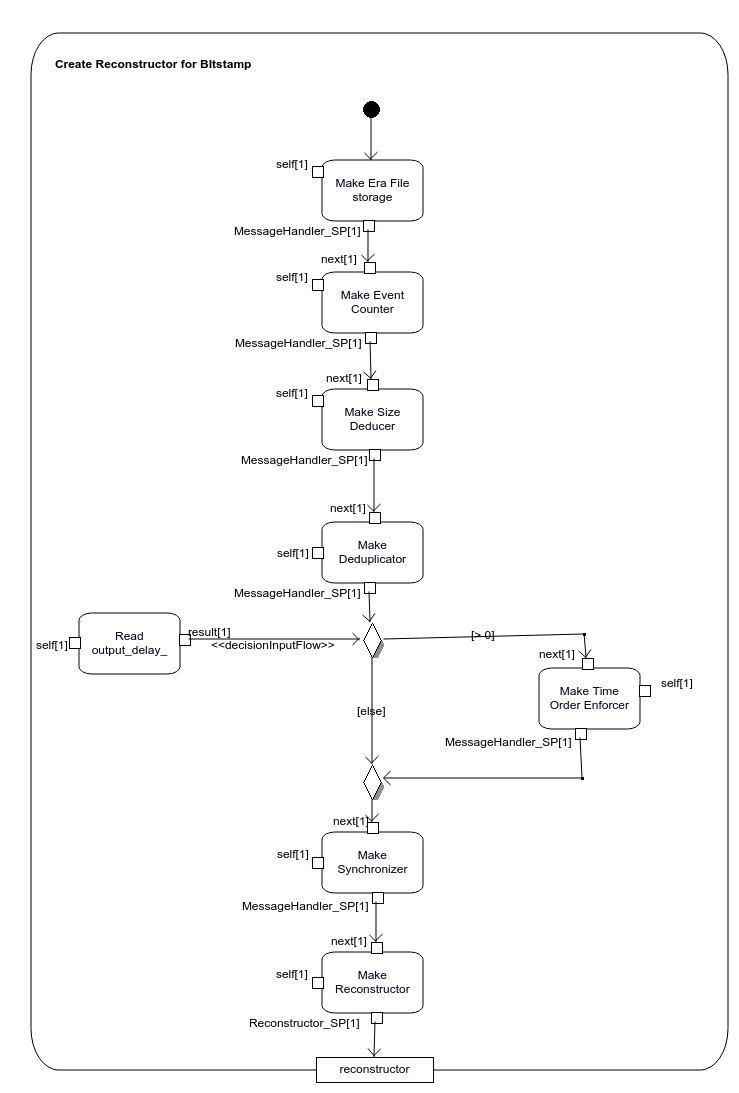
Figure 2.8: Specification of bitstamp::Capture::createReconstructor operation
2.2.3.2.3 Slice
2.2.3.2.4 Merge
2.2.3.2.5 Transmute
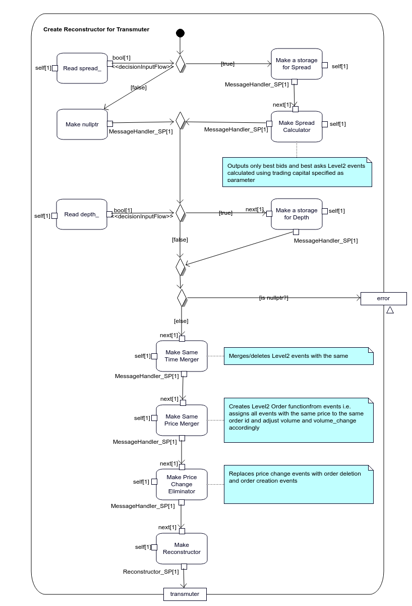
Figure 2.9: Specification of Transmute::createReconstructor operation
2.2.4 Acquire and process
This section provides specifications of acqureAndProcess operation of concrete classes shown on figure 2.6 in light-green. Note that both Receiver-derived classes share acquireAndProcess operation defined in Receiver class.
2.2.4.1 Receiver
Coinbase::Receiver and Bitstamp::Receiver classes inherit acquireAndProcess() method from Receiver class. Its activity diagram is shown on figure 2.10.
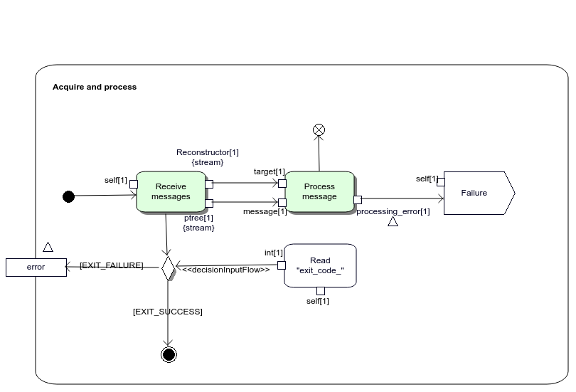
Figure 2.10: Specificationf of Receiver::acquireAndProcess() operation
2.2.4.2 Reader
Reader class has another acquireAndProcess() method. Its activity model is shown on figure 2.11.
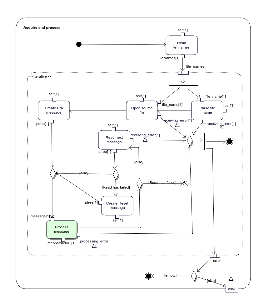
Figure 2.11: Specificationf of Reader::acquireAndProcess() operation
2.2.5 Receive messages
Action Receive messages on figure 2.10 is UML2 StartObjectBehaviorAction that starts execution of Receiver StateMachine shown on figure 2.12. The call is synchronous, so the execution of the Receive messages does not complete until the execution of Receiver StateMachine completes.
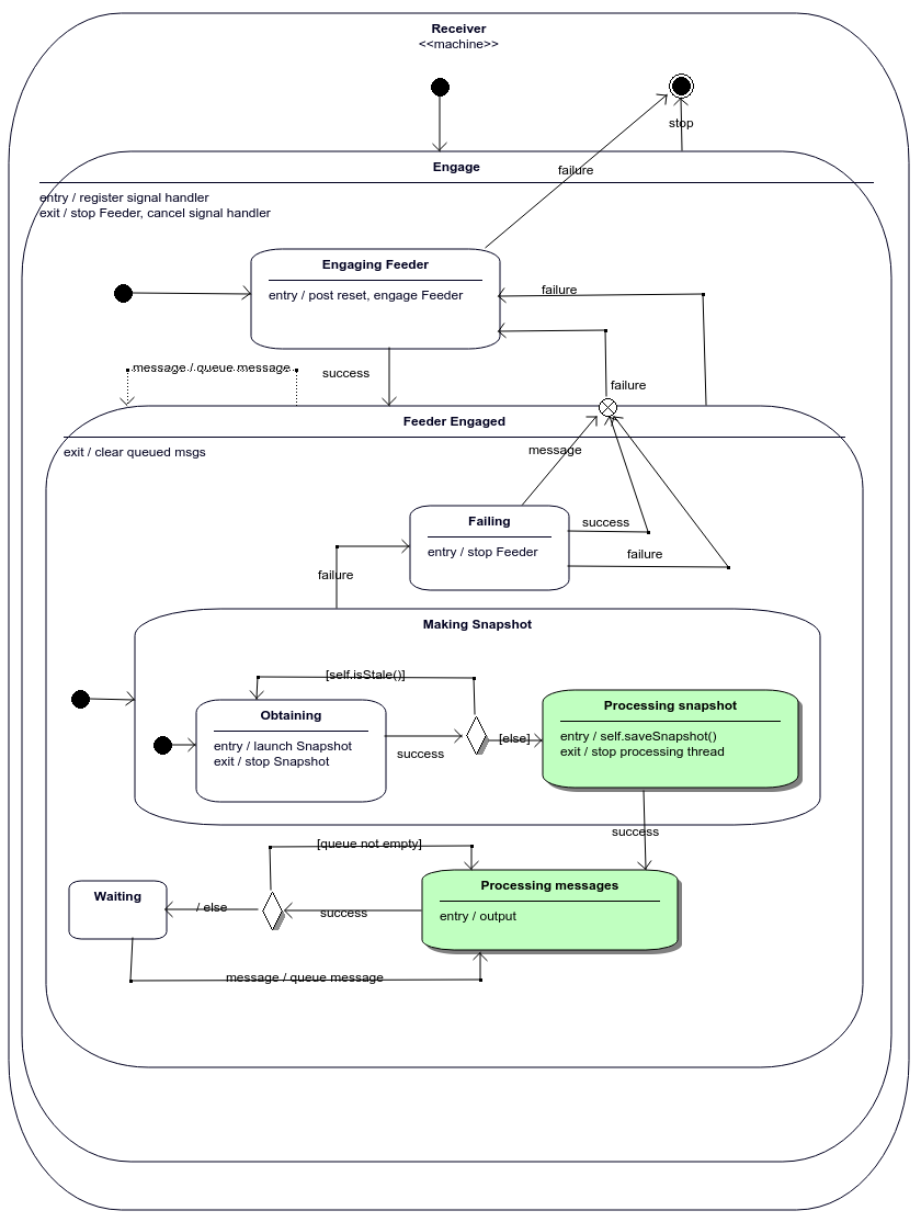
Figure 2.12: Processing snapshot and Processing messages states pass received portions of data asynchronously to an instance of Reconstructor (by calling operation Reconstructor::process() shown on figure 2.15) thereby the streaming of data between Receive messages and Process message on figure 2.10 is implemented.
Almost all exchanges provide two separate channels for receiving (i) a list of orders currently open on order book and (ii) order updates. In order to capture a dynamics of an order book one need to receive information from both channels and combine it. Feeder StateMachine shown on figure 2.13 deals with receiving order updates while Snapshot StateMachine shown on figure 2.14 is responsible for getting a list of orders currently open on order book.
Now look at figure 2.12 again. An entry behaviour of Engage.Engaging Feeder state launches Feeder StateMachine asynchronously. The latter sends “success” event as soon as it successfully subscribed for order updates and Receiver transitions to Engage.Feeder Engaged.Making Snapshot.Obtaining state. The state’s entry behaviour asynchronously launches Snapshot StateMachine shown on figure 2.14.
While Receiver remains in Engaged.Feeder Engaged.Making Snapshot state messages sent by Feeder are queued by internal transition activity on Receiver.Feeder Engaged state. As soon as Snapshot has received the snapshot, it sends Receiver “success” event and Receiver checks whether the snapshot and messages from Feeder cover the intersecting time periods or the snapshot is stale. In the latter case the snapshot is re-queried. Otherwise Receiver transitions to Processing snapshot state which asynchronously passes the snapshot to Reconstruct Order Book activity and upon receiveing “success” event transitions to Processing messages which asynchronously passes messages received from an exchange to Reconstruct Order Book. It is assumed that Receiver spends most of the time in this state.
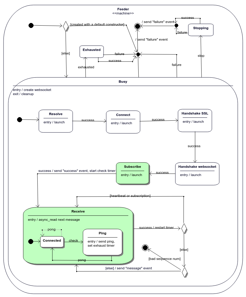
Figure 2.13: Transition success between Subscribe and Receive states sends “success” event to Receiver StateMachine. An entry behaviour of Receive state launches asynchronous read operation, whose successfull completion triggers success transition from Receive. If some service message (i.e. heartbeat, subscription) has arrived, it is processed locally. Otherwise “message” event is sent to Receiver.
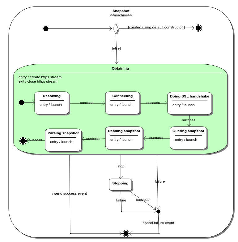
Figure 2.14: Snapshot StateMachine diagram.
2.2.6 Process message
Activity Process message shown on figure 2.15 is a specification of Reconstructor::process operation.
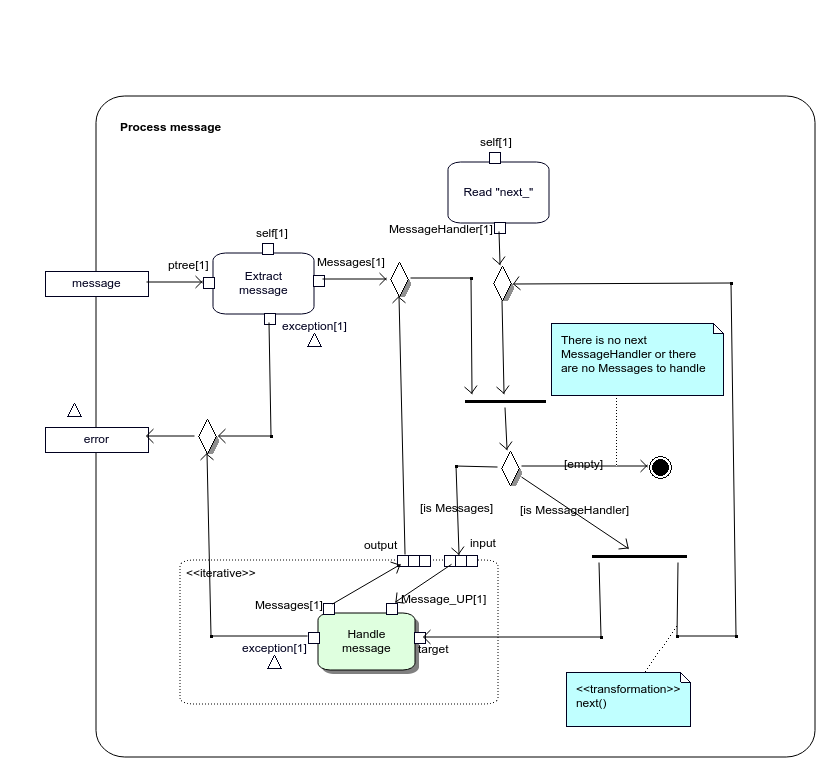
Figure 2.15: Specification of Reconstructor::process() operation that is called by Process message node
It takes an instance of Boost.PropertyTree container with an exchange-specific data as message parameter and passes it to Extract message action. The action creates then an instance of one of the exchange-independent class, derived from Message. Possible classes are shown in green on figure 2.16. The instance is returned in Messages container. The cointainer is a list of unique pointers Message_UP to Message-derived objects.
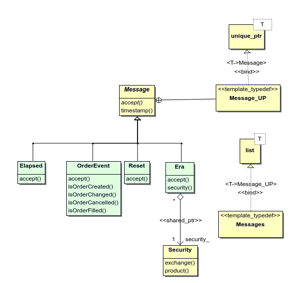
Figure 2.16: Extract returns an instance of class Messages
The further processing of messages by MessageHandlers is implemented using Chain of Responsibility pattern. Messages container is passed to ExpansionRegion of type “iterative” as input parameter as shown on figure 2.15. The region calls MessageHandler::handle operation on the instance of MessageHandler currently available within the region for each Message_UP in input. The outputs are combined and passed to the next MessageHandler returned by next transformation, if any (this instance becomes available for the next iteration). The cycle repeats until either input or next MessageHandler is empty.
When created, an instance of MessageHandler takes, as a constructor parameter, a shared pointer to the next MessageHandler which will receive messages as soon as MessageHandler being constructed has handled them. Thus the chain is static, i.e. it does not change depending on messages received.
The kind of processing performed by the chain of MessageHandlers depends on command being performed.
For command “capture” the chain performes so called data cleansing. According to (Rahm and Do 2000):
Data cleaning, also called data cleansing or scrubbing, deals with detecting and removing errors and inconsistencies from data in order to improve the quality of data.
It should be clear from the definition of order table 2.7 that not every set of order events as defined by 2.6 represents a valid order table. Similarly, not every set of orders represents valid LOB as defined by 2.15.
Data cleansing process receives a stream of order events (possible extended and/or incomplete i.e. order events as defined by 2.6 but with some additional and/or missing attributes), restores order functions from them and then restores LOB from order functions.
The exact list of MessageHandlers needed for that depends on exchange. The lists are described in section 2.2.3.2.
2.2.7 Handle message
UML2 Sequence Diagram of MessageHandler::handle() is shown on figure 2.17.
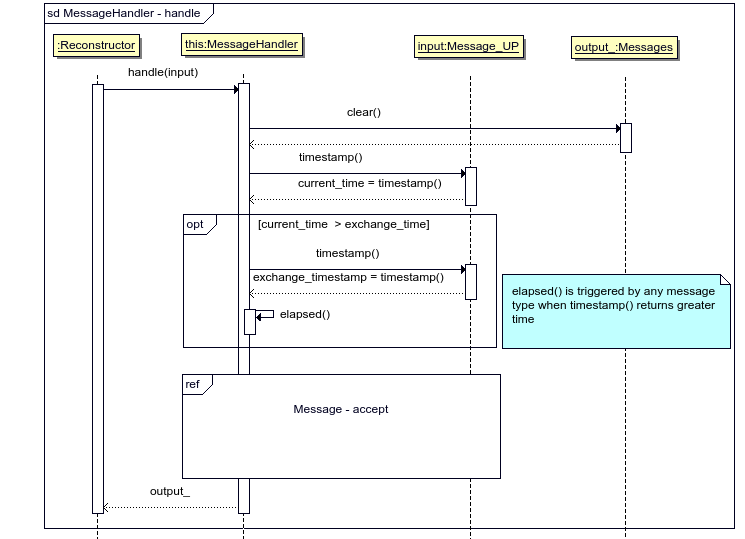
Figure 2.17: UML2 Sequence diagram showing a “happy path” trace of MessageHandler::handle() method.
Handling of messages by MessageHandler is implemented using Visitor pattern as shown by UML2 Sequence diagram on figure 2.18.
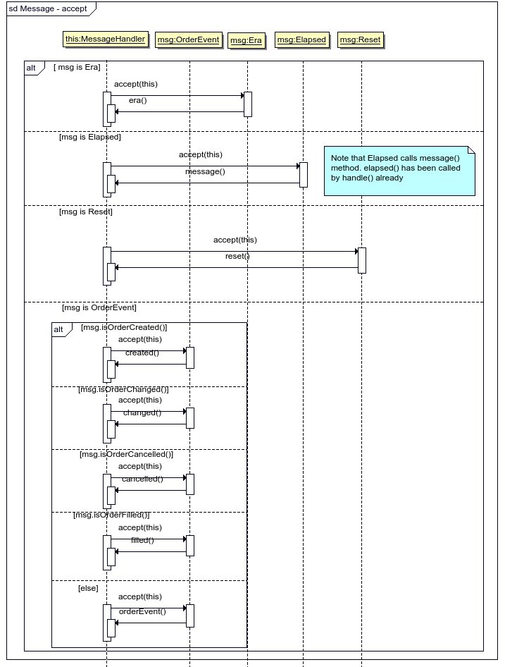
Figure 2.18: UML2 Sequence diagram showing various alternatives of traces for Message::accept() method. By default all MessageHandlers callback (i.e. era, message etc) just pass the message to output_ and it is expected that derived classes override the callbacks in order to do something useful. The message can be saved by MessageHandler instance in order to be processed later together with messages that follows.
The result of handle is a set of zero or more messages that are stored in output_ member variable that is an instance of Messages class shown on figure 2.16. MessageHandler will not produce output for a message when subsequent messages are required for handling. In this case the message will be kept within this particular MessageHandler instance between runs of Reconstructor::process() until enough subsequent messages have been received. Then all kept and handled messages are returned together, saved into output_ variable.
2.2.8 Output format
2.2.8.1 File
MessageHandler File saves the received events into files. Upon receiving of a message of class Era (see figure 2.16) File opens a new file called Era file and saves the subsequent OrderEvent messages there until obtaining Reset message when the handler closes Era file. File drops Elapsed messages silently.
Era file is CSV-file with one row per OrderEvent and its name is constructed from exchange, product and timestamp values carried by Era message. Row fields are described in the table 2.4 below.
| # | Field | Type | Description | Element |
|---|---|---|---|---|
| 1 | maker | UUID | an unique identification number of the order open on the order book | \(i\) |
| 2 | ordinal | long | A sequential number of the event for this order | \(k\) |
| 3 | timestamp | string | Time the event occurred, in ISO 8601 format, up to a second. Empty field means that the value is the same as in the previous event (previous row) | \(t_k^i\) |
| 4 | mks | int | Microseconds part of the time the event occurred, if different from zero; otherwise empty | \(t_k^i\) |
| 5 | timestamp_change | long long | Microseconds passed since the previous event, i.e. \(t_k^i - t_{k-1}^i\) if \(k\) is greater than 1 and \(t_k^i \neq t_{k-1}^i\); otherwise empty | |
| 6 | state | bool | 1, if the order is open on the order book after the event; otherwise empty | \(s_k^i\) |
| 7 | price | double | Price of the order | \(p_k^i\) |
| 8 | price_change | double | Price change since the previous event, i.e. \(p_k^i - p_{k-1}^i\) if \(k\) is greater than 1 and \(p_k^i \neq p_{k-1}^i\); otherwise empty | |
| 9 | volume | double | Volume of the order if different from zero; otherwise empty | \(v_k^i\) |
| 10 | volume_change | double | Change of the order’s volume since the previous event, i.e. \(v_k^i - v_{k-1}^i\) if \(k\) is greater than 1 and \(v_k^i \neq v_{k-1}^i\); otherwise empty | |
| 11 | trade | long long | If the event is originated by a trade it is an unique trade identification number; otherwise emtpy. Thus \(m_k^i \equiv\) trade isn’t empty | \(m_k^i\) |
| 12 | taker | UUID | If the event is originated by a trade, it is an unique identification number of the matched taker order; otherwise empty | |
| 13 | heard | int | Microseconds passed since the event occurred on the exchange till the application heard about it, if the event occured on the exchange; otherwise empty | |
| 14 | deleted | bool | 1, if the event’s been deleted (for example, it is a duplicate event); otherwise empty |